20180811a - Checking Kretz probe - client
#!/usr/bin/python
import spidev
import RPi.GPIO as GPIO
import time
import numpy as np
import matplotlib
import matplotlib.pyplot as plt
import json
import time
from pyUn0 import *
Setup

# Taggin this image accordingly
r = TagImage("P_20180811_190929.jpg","kretzaw145ba",x.iD,"setup","Connection of plugs to test")
Actions
Testing on the 3 coax cables there are in the head
for data in glob.glob("data/*.json"):
print data
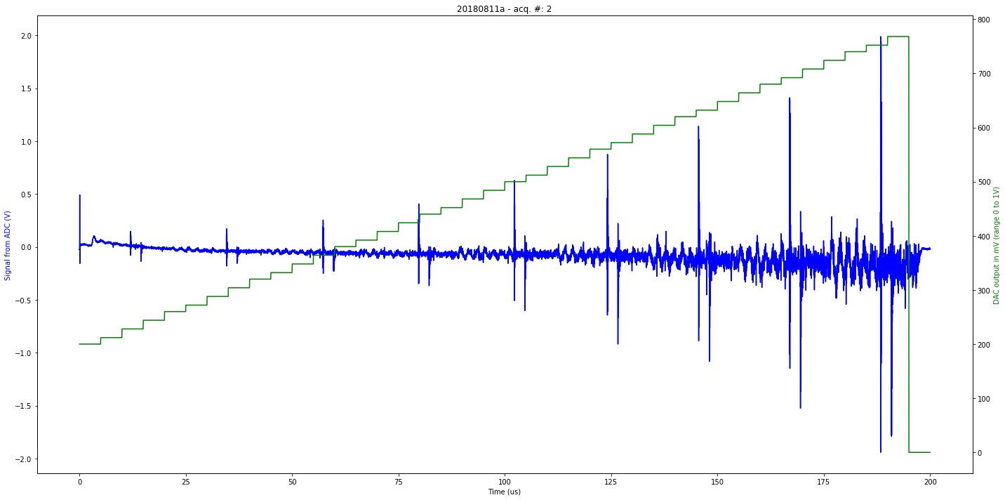
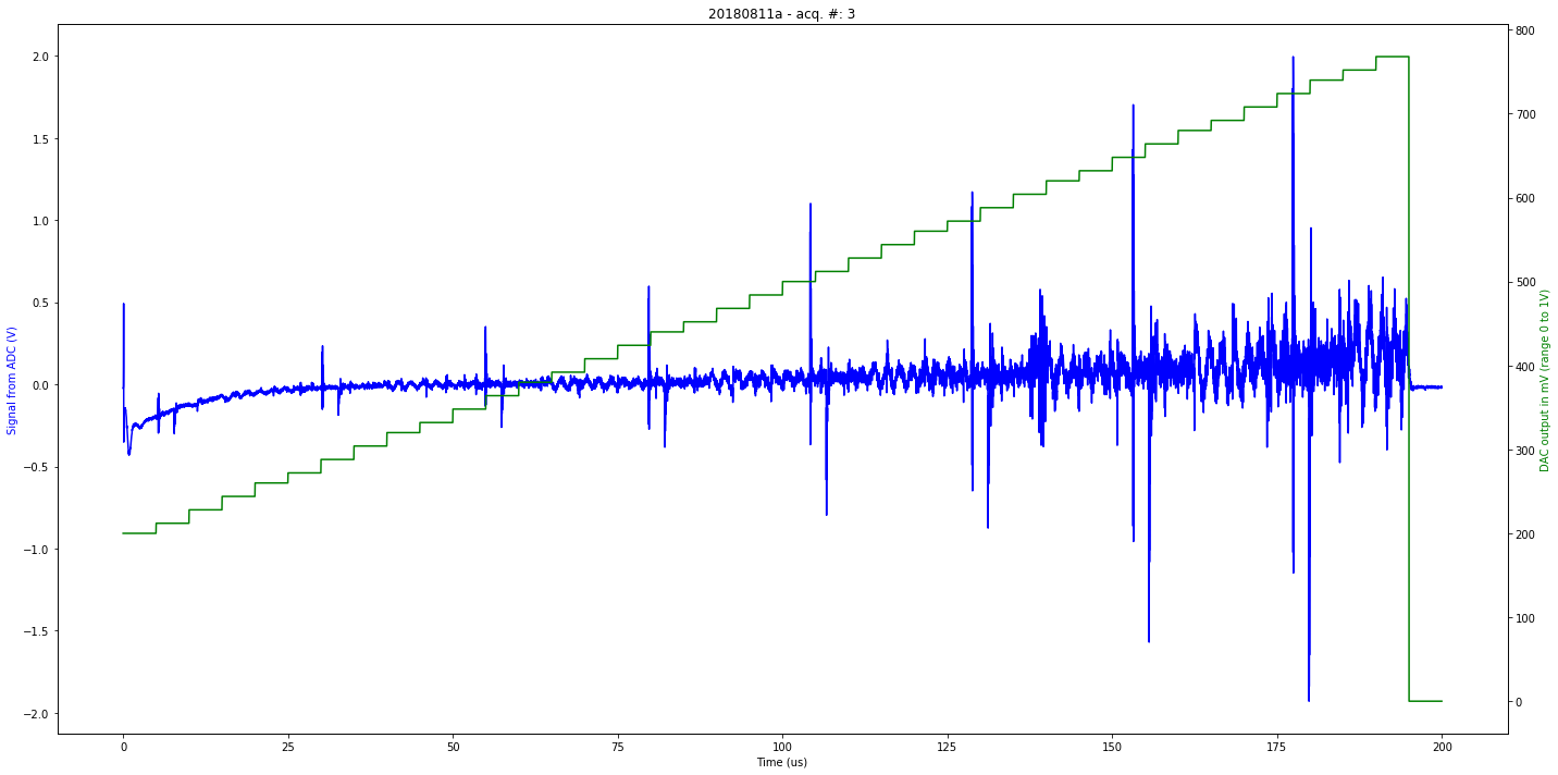
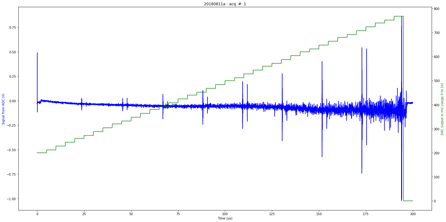
x = us_json()
x.JSONprocessing(data)
x.mkImg()
#x.PlotDetail(0,100,125)
#x.SaveNPZ()
print x.Nacq
data/20180811a5.json
1
data/20180811a6.json
1
data/20180811a4.json
1
data/20180811a7.json
1
data/20180811a2.json
1
data/20180811a3.json
1
data/20180811a1.json
1
Checking data
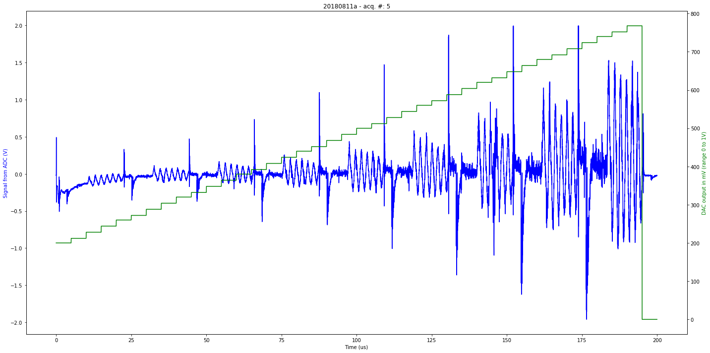
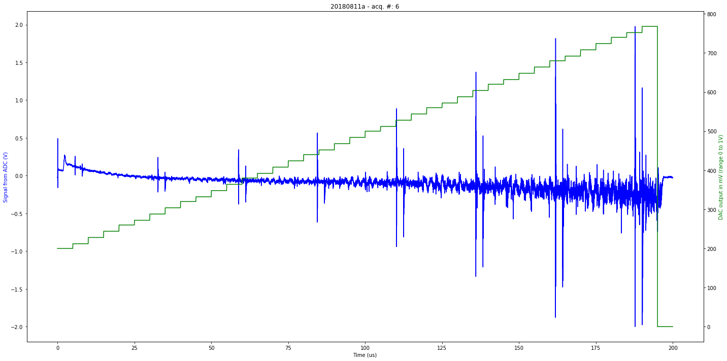
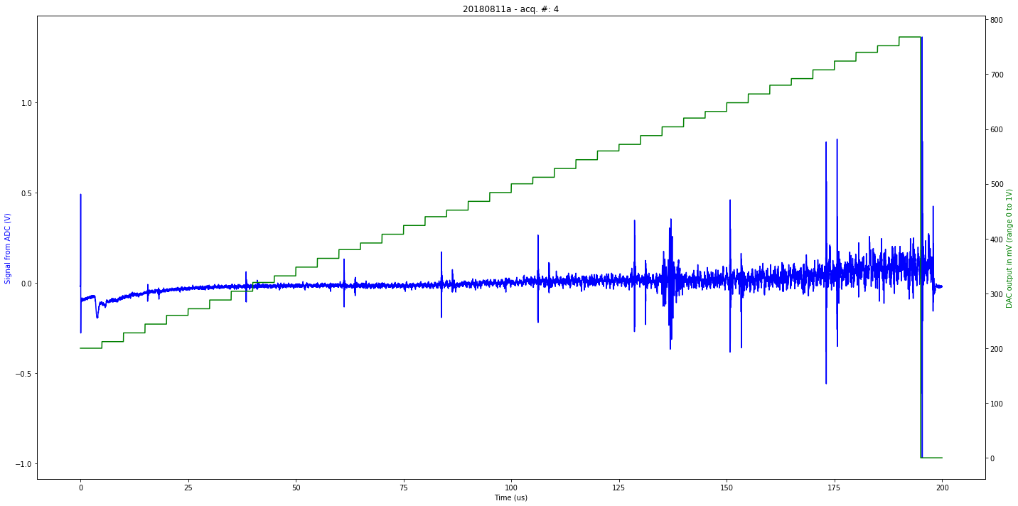
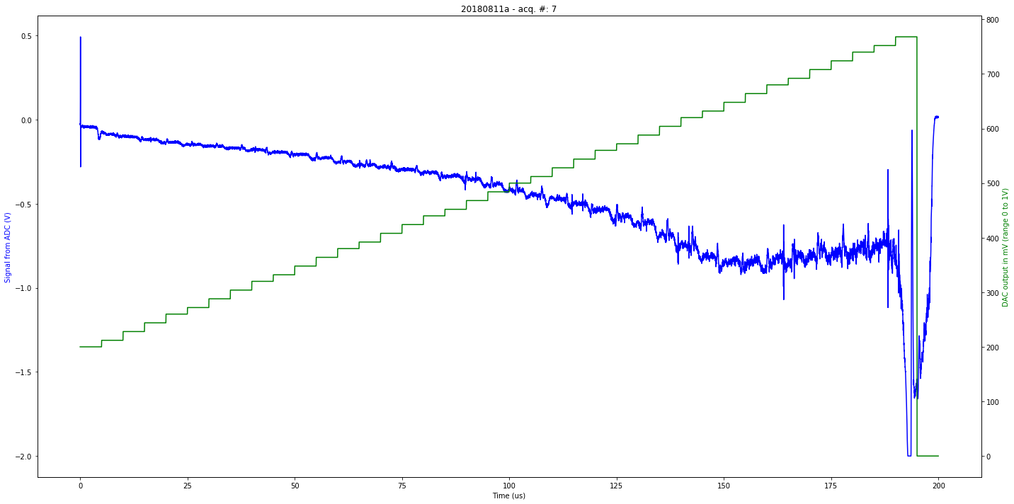
Setup: the probe was in water, piezo facing bottom of glass, at around 10cm
It seems only the data files 3 and 4 have a signal corresponding to this distance.
x = us_json()
x.JSONprocessing("data/20180811a3.json")
y = us_json()
y.JSONprocessing("data/20180811a4.json")
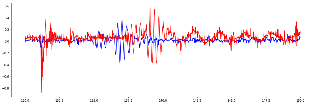
Checking lines between 130 and 150 us
A = 130
B = 150
plt.figure(figsize=(15,5))
plt.plot(y.t[64*A:64*B],y.tmp[64*A:64*B],"b")
plt.plot(x.t[64*A:64*B],x.tmp[64*A:64*B],"r")

plt.tight_layout()
FileName = x.iD+"-"+str(x.N)+"first-lines-rawsignal.jpg"
plt.savefig(FileName)
plt.show()
TagImage(FileName,"kretzaw145ba",x.iD,"lines",y.description)
1
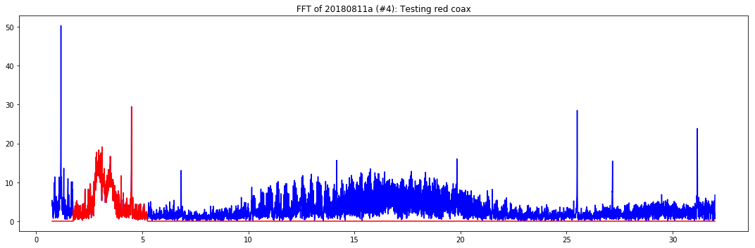
Filtering
plt.figure(figsize=(15,5))
plt.plot(y.FFT_x[150:y.len_line/2],np.abs(y.FFT_y[150:y.len_line/2]),"b")
plt.plot(y.FFT_x[150:x.len_line/2],np.abs(y.FFT_filtered[150:x.len_line/2]),"r")
plt.title ("FFT of "+y.iD +" (#"+str(y.N)+"): " +y.description)

plt.tight_layout()
FileName = x.iD+"-"+str(x.N)+"first-lines-fft.jpg"
plt.savefig(FileName)
plt.show()
TagImage(FileName,"kretzaw145ba",x.iD,"fft",y.description)
1
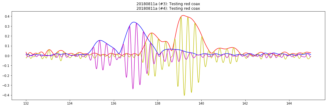
Let's see, once filtered around 3.5MHz
Lets see if we see anything..
A = 132
B = 145
plt.figure(figsize=(15,5))
plt.plot(x.t[64*A:64*B],x.EnvHil[64*A:64*B],"r")
plt.plot(x.t[64*A:64*B],x.SignalFiltered[64*A:64*B]+1/2,"y")
plt.plot(y.t[64*A:64*B],y.EnvHil[64*A:64*B],"b")
plt.plot(y.t[64*A:64*B],y.SignalFiltered[64*A:64*B],"m")
plt.title (  x.iD +" (#"+str(x.N)+"): " + x.description +"\n"+y.iD +" (#"+str(y.N)+"): " +y.description)

plt.tight_layout()
FileName = x.iD+"-"+str(x.N)+"first-lines.jpg"
plt.savefig(FileName)
plt.show()
TagImage(FileName,"kretzaw145ba",x.iD,"lines",y.description)
1
Nexteps
Check the "20180430a" experiment for the "ServoControl.ino" file.
Idea is to have STEPs lines: TopTurn1 + TopTurn2:
- STEP high
- SPI 0xFF, 0xCounter
- delay (to be fixed)
- STEP low
- SPI 0x00, 0xCounter
- delay (to be fixed)
This way, there will be cycle counter, and an line with some info:
- Cycle Counter (2 bits)
- MOSI + Clock (2 bits)
Along with 2bits headers, and 10 bits data, we reach our allowance of 16bits words for each point.
Cheatsheet: keys for us_json instances
x.__dict__.keys()
['IDLine',
 'FFT_x',
 'FFT_y',
 'single',
 'experiment',
 'piezo',
 'FFT_filtered',
 'processed',
 'tmp',
 'parameters',
 'len_line',
 'LengthT',
 'Nacq',
 'iD',
 't',
 'description',
 'TT2',
 'TT1',
 'EnvHil',
 'N',
 'V',
 'len_acq',
 'firmware_md5',
 'f',
 'Registers',
 'SignalFiltered',
 'tdac']